Περιγραφή¶

TensorFlow is an end-to-end open source platform for machine learning

TensorFlow 2.11.1 (CPU only)¶

Το script υποβολής μίας εργασίας που χρησιμοποιεί το TensorFlow θα έχει την ακόλουθη μορφή:

SLURM submission script

TensorFlow-2.11.1-case.sh

#!/bin/bash
#SBATCH --job-name=TensorFlow-2.11.1-case
#SBATCH --partition=batch
#SBATCH --time=10:00

# conda commands
module load gcc/10.2.0 miniconda3/4.10.3-rflbhqow
source $CONDA_PROFILE/conda.sh
conda activate /mnt/apps/custom/conda/tensorflow-cpu-2.11.1
export PATH=$CONDA_PREFIX/bin:$PATH
export LD_LIBRARY_PATH=$LD_LIBRARY_PATH:$CONDA_PREFIX/lib

# code to be executed
python3 tensorflow_example.py

Στο $HOME μας στο login node, δημιουργούμε ένα νέο φάκελο όπου τοποθετούμε τα αρχεία εισόδου και το script υποβολής της εργασίας, έστω TensorFlow-2.11.1-case.sh.

# mkdir TensorFlow-2.11.1-case
# cd TensorFlow-2.11.1-case

Για το συγκεκριμένο παράδειγμα θα χρησιμοποιήσουμε το "Hello World" example που δίνεται εδώ.

TensorFlow example

import tensorflow as tf
mnist = tf.keras.datasets.mnist

(x_train, y_train),(x_test, y_test) = mnist.load_data()
x_train, x_test = x_train / 255.0, x_test / 255.0

model = tf.keras.models.Sequential([
  tf.keras.layers.Flatten(input_shape=(28, 28)),
  tf.keras.layers.Dense(128, activation='relu'),
  tf.keras.layers.Dropout(0.2),
  tf.keras.layers.Dense(10, activation='softmax')
])

model.compile(optimizer='adam',
              loss='sparse_categorical_crossentropy',
              metrics=['accuracy'])

model.fit(x_train, y_train, epochs=5)
model.evaluate(x_test, y_test)

Η υποβολή της εργασίας γίνεται με την εντολή sbatch <filename.sh> ως εξής:

# sbatch TensorFlow-2.11.1-case.sh

Παρακολουθούμε με την εντολή squeue την εξέλιξη της εργασίας.

Eφόσον η εργασία έχει εκκινήσει μπορούμε να ελέγχουμε την πρόοδο της επίλυσης μέσω των αρχείων εξόδου. Π.χ.:

# tail -f *.out

TensorFlow 2.11.1 + GPU support (`Ampere` partition)¶

Το script υποβολής μίας εργασίας που χρησιμοποιεί το TensorFlow με GPU support θα έχει την ακόλουθη μορφή:

SLURM submission script

#!/bin/bash
#SBATCH --job-name=TensorFlow-2.11.1-case
#SBATCH --partition=ampere
#SBATCH --gres=gpu:1
#SBATCH --time=10:00

# conda commands
module load centos8 gcc/11.2.0 miniconda3/4.10.3
source $CONDA_PROFILE/conda.sh
conda activate /mnt/apps/custom/conda/tensorflow-2.11.1-ampere
export LD_LIBRARY_PATH=$LD_LIBRARY_PATH:$CONDA_PREFIX/lib
export XLA_FLAGS="--xla_gpu_cuda_data_dir=$CONDA_PREFIX/lib"

# code to be executed
python3 -c "import tensorflow as tf; print(tf.config.list_physical_devices('GPU'))"
python3 tensorflow_tutorial.py

Θα χρησιμοποιήσουμε εδώ ένα παράδειγμα από το TensorFlow 2 quickstart tutorial for beginners:

TensorFlow beginners tutorial example

import tensorflow as tf
print("TensorFlow version:", tf.__version__)

# ## Load a dataset
# 
# Load and prepare the [MNIST dataset](http://yann.lecun.com/exdb/mnist/). The pixel values of the images range from 0 through 255. Scale these values to a range of 0 to 1 by dividing the values by `255.0`. This also converts the sample data from integers to floating-point numbers:

mnist = tf.keras.datasets.mnist

(x_train, y_train), (x_test, y_test) = mnist.load_data()
x_train, x_test = x_train / 255.0, x_test / 255.0

# ## Build a machine learning model
# 
# Build a `tf.keras.Sequential` model:

model = tf.keras.models.Sequential([
  tf.keras.layers.Flatten(input_shape=(28, 28)),
  tf.keras.layers.Dense(128, activation='relu'),
  tf.keras.layers.Dropout(0.2),
  tf.keras.layers.Dense(10)
])

# For each example, the model returns a vector of [logits](https://developers.google.com/machine-learning/glossary#logits) or [log-odds](https://developers.google.com/machine-learning/glossary#log-odds) scores, one for each class.

predictions = model(x_train[:1]).numpy()
predictions

# The `tf.nn.softmax` function converts these logits to *probabilities* for each class: 

tf.nn.softmax(predictions).numpy()

# Define a loss function for training using `losses.SparseCategoricalCrossentropy`:

loss_fn = tf.keras.losses.SparseCategoricalCrossentropy(from_logits=True)


# The loss function takes a vector of ground truth values and a vector of logits and returns a scalar loss for each example. This loss is equal to the negative log probability of the true class: The loss is zero if the model is sure of the correct class.
# 
# This untrained model gives probabilities close to random (1/10 for each class), so the initial loss should be close to `-tf.math.log(1/10) ~= 2.3`.

loss_fn(y_train[:1], predictions).numpy()


# Before you start training, configure and compile the model using Keras `Model.compile`. Set the [`optimizer`](https://www.tensorflow.org/api_docs/python/tf/keras/optimizers) class to `adam`, set the `loss` to the `loss_fn` function you defined earlier, and specify a metric to be evaluated for the model by setting the `metrics` parameter to `accuracy`.

model.compile(optimizer='adam',
              loss=loss_fn,
              metrics=['accuracy'])


# ## Train and evaluate your model
# 
# Use the `Model.fit` method to adjust your model parameters and minimize the loss: 

model.fit(x_train, y_train, epochs=100)

# The `Model.evaluate` method checks the model's performance, usually on a [validation set](https://developers.google.com/machine-learning/glossary#validation-set) or [test set](https://developers.google.com/machine-learning/glossary#test-set).

model.evaluate(x_test,  y_test, verbose=2)


# The image classifier is now trained to ~98% accuracy on this dataset. To learn more, read the [TensorFlow tutorials](https://www.tensorflow.org/tutorials/).

# If you want your model to return a probability, you can wrap the trained model, and attach the softmax to it:

probability_model = tf.keras.Sequential([
  model,
  tf.keras.layers.Softmax()
])

probability_model(x_test[:5])

# ## Conclusion
# 
# Congratulations! You have trained a machine learning model using a prebuilt dataset using the [Keras](https://www.tensorflow.org/guide/keras/overview) API.
# 
# For more examples of using Keras, check out the [tutorials](https://www.tensorflow.org/tutorials/keras/). To learn more about building models with Keras, read the [guides](https://www.tensorflow.org/guide/keras). If you want learn more about loading and preparing data, see the tutorials on [image data loading](https://www.tensorflow.org/tutorials/load_data/images) or [CSV data loading](https://www.tensorflow.org/tutorials/load_data/csv).
#

CUDA packages versions in environment:

cuDNN: 8.4.1.50
CUDA toolkit: 11.8.0
CUDA nvcc: 12.1.66

TensorFlow 2.11.1 + GPU support (`GPU` partition)¶

Το script υποβολής μίας εργασίας που χρησιμοποιεί το TensorFlow με GPU support θα έχει την ακόλουθη μορφή:

SLURM submission script

#!/bin/bash
#SBATCH --job-name=TensorFlow-2.11.1-case
#SBATCH --partition=gpu
#SBATCH --gres=gpu:1
#SBATCH --time=10:00

# conda commands
module load gcc/12.2.0 miniconda3/4.10.3
source $CONDA_PROFILE/conda.sh
conda activate /mnt/apps/custom/conda/tensorflow-gpu-2.11.1
export LD_LIBRARY_PATH=$LD_LIBRARY_PATH:$CONDA_PREFIX/lib
export XLA_FLAGS="--xla_gpu_cuda_data_dir=$CONDA_PREFIX/lib"


# code to be executed
python3 tensorflow_gpu_example.py

Θα χρησιμοποιήσουμε εδώ ένα παράδειγμα από το GPU guide documenation του TensorFlow:

TensorFlow GPU example

import tensorflow as tf
print("Num GPUs Available: ", len(tf.config.list_physical_devices('GPU')))

tf.debugging.set_log_device_placement(True)

# Create some tensors
a = tf.constant([[1.0, 2.0, 3.0], [4.0, 5.0, 6.0]])
b = tf.constant([[1.0, 2.0], [3.0, 4.0], [5.0, 6.0]])
c = tf.matmul(a, b)

print(c)

TensorFlow 2.0.0¶

Παράδειγμα χρήσης¶

Το script υποβολής μίας εργασίας που χρησιμοποιεί το TensorFlow θα έχει την ακόλουθη μορφή:

SLURM submission script

#!/bin/bash
#SBATCH --job-name=TensorFlow-2.0.0-case
#SBATCH --partition=batch
#SBATCH --time=10:00

# conda commands
module load intel miniconda3
source $CONDA_PROFILE/conda.sh
conda activate /mnt/apps/prebuilt/conda/3/envs/tensorflow
export PATH=$CONDA_PREFIX/bin:$PATH

# code to be executed
python tensorflow_example.py

Γραφικό Περιβάλλον TensorBoard¶

Στη συστοιχία διατίθεται το γραφικό περιβάλλον του TensorBoard server για την παρακολούθηση εργασιών tensorflow. Για να χρησιμοποιήσουμε το γραφικό περιβάλλον του TensorBoard στην συστοιχία μπορούμε να επισκεφτούμε με έναν browser την σελίδα: https://hpc.auth.gr και να ακολουθήσουμε τα παρακάτω βήματα:

Από το menu επιλέγουμε Interactive Apps -> TensorBoard
Στην συνέχεια επιλέγουμε στην φόρμα τον κατάλογο των logs (logdir) που θέλουμε να παρακολουθήσουμε με το TensorBoard και τυχόν άλλα ορίσματα γραμμής εντολών για το TensorBoard.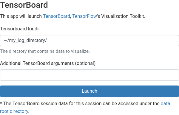
Eφόσον η εργασία ξεκινήσει, μπορούμε να επιλέξουμε Launch TensorBoard.

Προσθήκη επιπλέον πακέτων στο environment¶

Πολλές φορές χρειαζόμαστε πακέτα πέραν όσων περιέχονται στο έτοιμο environment για το TensorFlow. Τότε θα πρέπει να αντιγράψουμε τοπικά το εν λόγω περιβάλλον ώστε να μπορούμε έπειτα να το επεξεργαστούμε. Συγκεκριμένα, ας πάρουμε για παράδειγμα το TensorFlow/2.11.1 για CPU, για το οποίο θα ενεργοποιούσαμε το περιβάλλον /mnt/apps/custom/conda/tensorflow-cpu-2.11.1. Στη θέση της εντολής

# conda activate /mnt/apps/custom/conda/tensorflow-cpu-2.11.1

θα χρησιμοποιήσουμε τις εντολές

# conda create --clone /mnt/apps/custom/conda/tensorflow-cpu-2.11.1 -n newEnv
# conda activate newEnv

οι οποίες δημιουργούν και ενεργοποιούν ένα νέο περιβάλλον newEnv στο φάκελο όπου βρισκόμαστε. Το newEnv είναι όμοιο με το έτοιμο περιβάλλον για το TensorFlow και μπορούμε πλέον να το διαμορφώσουμε όπως θέλουμε, δίνοντας conda install <όνομα πακέτου> για τα πακέτα που χρειαζόμαστε.

Περισσότερες πληροφορίες για τη χρήση του conda θα βρείτε εδώ.

Περιγραφή¶

TensorFlow 2.11.1 (CPU only)¶

TensorFlow 2.11.1 + GPU support (Ampere partition)¶

TensorFlow 2.11.1 + GPU support (GPU partition)¶

TensorFlow 2.0.0¶

Παράδειγμα χρήσης¶

Γραφικό Περιβάλλον TensorBoard¶

Προσθήκη επιπλέον πακέτων στο environment¶

TensorFlow 2.11.1 + GPU support (`Ampere` partition)¶

TensorFlow 2.11.1 + GPU support (`GPU` partition)¶